HFT Engine Latency - Part 1

Latency of an actual C++ engine

Sep 06, 2025

When building an systematic trading engine, performance is always a central concern. Among the various performance metrics, latency stands out as the most important. It measures how quickly a trading engine can process market data, evaluate trading logic, and fire out an order. Performing these critical actions at high speed can directly influence execution quality, allows for backtests to run faster, and ties directly to strategy profitability.

In this article we are going to examine the latency of Apex, a C++ trading and backtest engine. Although Apex has not initially been designed as a low latency platform, it will still have a latency that we would should be able to measure, and monitor as later improvements are made.

Thinking About Latency

Tick to Trade

If latency is the time taken for the engine to complete some work, then we must ask: which tasks are included — when is the timer started, and when does it stop?

A natural place to start at is with the full round-trip latency. This is illustrated in the figure below: the engine receives a market data update — for example, a trade print or a level-1 quote change — and responds by generating and transmitting an order to the exchange. This complete “tick-to-trade” chain treats the trading engine as a black box, ignoring its internal structure. If we can capture the time at which market data enters the server and the time at which the order leaves the server, we obtain the full tick-to-trade response latency, T1 - T0.

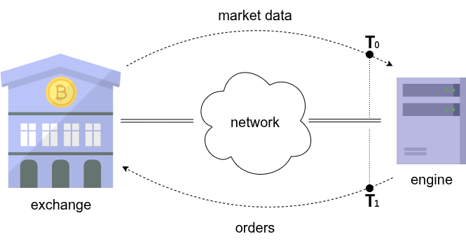
Unfortunately, capturing this measurement is not easy to perform. It requires recording and decoding activity at the network level, where market data and order messages (in the form of UDP or TCP packets) flow between the switch and the server. In professional high-frequency environments, specialised hardware is often used for this purpose, such as Corvil network appliances.

Internal Latency

Instead of network based tick-to-trade, a more practical starting point is to look at internal software latency. This is the time taken by only the trading application: the sequence of tasks that occur when a tick arrives into the engine, is processed, and results in an order being generated. Time spent on the network, in the network card and in the OS, are excluded. How long do these internal steps take from input to decision?

Capturing internal latency is far more doable. Rather than relying on external packet capture, we can instrument the engine code directly, placing high-resolution timing points at critical milestones. This approach is more informative than measuring only overall tick-to-trade latency, since it reveals which subsystems dominate processing time and therefore guides targeted optimisation.

The next figure shows a fairly typical sequence of events for a tick based trading engine (in this case the engine has direct links to the exchange). An inbound flow sees market data packets arrive off the network, entering into the application by successive socket reads. These raw network bytes might then require framing/security protocol decoding (such as TLS & WebSocket). Then we have actual raw exchange data, which is then parsed to transform it into the native data structures of the application. Finally an internal model state is updated; in the case of a market data tick (such as a trade, or order book), a suitable market object is identified and updated appropriately.

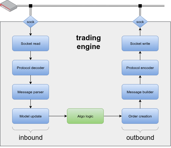
The strategy logic is now notified that the model has been updated, and makes a decision to send an order (or perhaps cancel a live order). The diagram shows this strategy section in a different colour, which is to illustrate that often the strategy logic (green) and engine components (blue), are often different sub-projects.

Once the strategy has made the decision to trade, the outbound flow commences. This sort of mirrors the preceding inbound flow in reverse First an engine order object is created, collecting the details of the order (such as instrument, price and quantity). This is then used to build the order message required by the exchange protocol. This exchange message then needs to be packaged into the framing/security protocol, before finally being written to the socket using a transport protocol, typically TCP.

By breaking down the flow into these sections, we can try to insert timestamp collection code at each step. For example, we can capture the time when data came off the socket, and the time when data was written to the socket, and from there we can determine overall internal tick-to-trade latency.

Apex Inbound Latency

The focus of this present study is on the inbound pathway, not yet the full internal tick-to-trade journey. By narrowing scope we can capture meaningful latency measurements without needing to complete the outbound flow, which requires generating large numbers of orders. This approach has practical advantages: it allows us to measure latency in any market data application, even in cases where no trading occurs.

Additionally, the inbound path — from tick arrival to model update — is the hottest pathway in the engine. It is invoked millions of times per day, whereas the outbound order path is comparatively rare. Optimising this inbound pipeline therefore has immediate, broad impact on responsiveness.

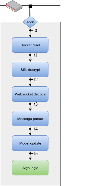
The following figure illustrates the exact locations where we will collect timing measurements along this path:

t0: when data is ready to be read from the socket.
t1: after the socket read completes.
t2: after SSL/TLS decryption.
t3: after each WebSocket message has been decoded.
t4: after the raw exchange message (JSON) has been parsed.
t5: after the market data model has been updated with the parsed information.

This breakdown allows for latency attribution to distinct stages: transport, security, protocol, parsing, and model update. With these granular measurements, we not only observe total inbound latency but can also identify which specific operations dominate processing time. That insight is critical for guiding later optimisation efforts.

Capture

Now that we have decided what to capture, the next step is to add timing capture code. This is where implementation details start to matter: we must decide how to measure latency inside the engine, and how to export those measurements for later analysis.

There are several ways to add timing instrumentation to code, depending on the clock facilities provided by the operating system. Each method has different performance characteristics. Importantly, inserting instrumentation itself adds a small performance overhead, so there is often a trade-off between precision, speed and convenience. For this initial investigation, we are primarily interested in obtaining baseline latency numbers, so we take the simplest approach: calling the system real-time clock. Latency improvements and finer-grained measurement can always be layered in step by step.

The following code snippet shows how timing is captured. In this example, a timestamp is taken after the engine is notified that socket data is available to be read:

int nfds = ::poll(&fds[0], fds.size(), timeout);

at_io.mark(); // timestamp when data can be read

Shortly later, after the actual read completes, we capture the next timestamp:

nread = ::read(s->fd, s->recv_buf(), s->recv_space());
s->tlog.at_io = at_io;
s->tlog.at_read.mark();  // capture time after socket read

The mark() function is a thin wrapper around clock_gettime using CLOCK_REALTIME. While this is not the fastest or most precise clock available on Linux, it is a reasonable starting point for initial measurements. Later iterations can switch to faster monotonic clocks or CPU clock cycles, if required.

The timestamps associated with the current market data event are stored in a timing log. Once the inbound stack arrives at the model update (t5), the full timing log is written to a memory mapped file. Using a memory-mapped file rather than direct logging helps to reduce I/O overhead, and it places all records in a central location for later ease of analysis.

Results

To generate data, the engine is compiled in release mode and configured to subscribe to several Binance Futures symbols (BTCUSDT, ETHUSDT, SOLUSDT, ADAUSDT). It is run for several hours, capturing around 16 million ticks (a mix of trades and level-1 updates). Tests are performed on commodity hardware: a 3.40 GHz Intel Core i7-6700 CPU, locked at maximum frequency to avoid down-clocking during idle periods, which would otherwise affect latency measurement

The following table shows latency results for each checkpoint. Each latency value is calculated by subtracting two successive timestamps. For example, s4 (after JSON parsing) is the difference between t4 and t3. For each measurement, we report min, max, mean, and various percentiles.

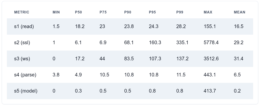
When reviewing a performance table like this, the question is: which numbers matter most? The P50 gives the median, while P95 and P99 point to worst performance. The max represents the absolute worst case, but large outliers are often discounted since they may result from unrelated system or network activity.

At P50, the cumulative inbound latency is around 50 µs. That’s a solid baseline for an engine not explicitly designed or tuned for low latency (though it is C++ and works directly with sockets). At the tail, performance significantly degrades, reaching a few hundred microseconds at P95/P99.

A few observations stand out:

WebSocket parsing (s3): Latency grows as messages further back in a batch wait for earlier messages to be decoded and fully processed. Higher values at the higher percentiles reflect queuing effects rather than engine inefficiency.
Socket poll → read (s1): This gap is surprisingly high, at over 20 µs, even though the engine does very little between these two points.
TLS decryption (s2): At P75, the cost is modest (≈7 µs), but at P99 it’s above 300 µs, which is very costly. However this may be linked to message size effects, where large batches arriving in a single read require more decryption work.

Overall, the results show a reasonable starting point, but also highlight areas where tuning and optimisation could bring significant improvements.

Summary

We have taken an initial look at the latency considerations of tick based trading applications, and obtained measurements for the C++ trading & backtest engine Apex.

Apex was not initially designed for low latency, so these results serve as a baseline. As improvements are introduced, we can compare back to this baseline to validate whether changes deliver real performance gains. This process should always be evidence-driven: observe, hypothesise, experiment, confirm, implement — and repeat.

Despite not being built with high performance as a primary goal, Apex shows a promising starting point. The median inbound tick-to-model latency is around 50 µs, which is respectable. However, performance at higher percentiles is much weaker, reaching several hundred microseconds.

Next steps will focus on improving inbound message latency and extending instrumentation to the outbound path, so that we can measure full internal tick-to-trade latency.